Efficiency

• quickly write, revise, run, and revisit your code

Transparency

• let others see & understand what you're doing

Reproducibility

• enable anyone to run your analyses

• implement each idea just once
• change data or methods freely
• handle more data & complexity
• run on clusters/cloud
• share with others
• share with your future self

Readable

• readable code
• traceable data flow

Self-contained

• complete from data to reports
• dependencies are included or public & documented

Incorruptible

• judicious redundancy
• code versioning
• automated data flow

• comments on goals & rationale
• meaningful variable names
• meaningful white space
• clarity via conciseness
• decomposition
• don't repeat yourself

Exhibit A

for(i in seq_len(n)[-1]) {
mu[i,d]<-  X[i-1, d]+((GPP[d]/z)*(light[i,d]/(sum(light[,d]))))+ (ER[d]*0.006944/z)-
  (K[d]/(600/(1800.6-(temp[i,d]*120.1)+(3.7818*temp[i,d]^2)-(0.047608*temp[i,d]^3)))^
-0.5) * 0.0069444*(  ((exp(2.00907 + 3.22014 * (log((298.15-temp[i,d]) / (273.15 + 
temp[i,d]))) + 4.0501 * (log((298.15 - temp[i,d]) / (273.15 + temp[i,d]))) ^ 2 + 
4.94457 * (log((298.15 - temp[i,d]) / (273.15 + temp[i,d]))) ^ 3 - 0.256847 * 
  (log((298.15 - temp[i,d]) / (273.15 + temp[i,d]))) ^ 4 + 3.88767 * (log((298.15 - 
temp[i,d]) / (273.15 + temp[i,d]))) ^ 5)) * 1.4276 * bp / 760) *satcor-X[i-1,d] )}

Exhibit B

# Compute the O2-specific reaeration coefficient for each timestep
K <- convert_k600_to_kGAS(K600.daily, temperature=temp.water, gas="O2") * frac.D

# Dissolved oxygen (DO) at each time i is a function of DO at time i-1 plus
# productivity, respiration, and reaeration
for(i in seq_len(n)[-1]) {
  DO.mod[i] <- 
    DO.mod[i-1] +
    GPP[i] + 
    ER[i] - 
    K[i] * (DO.sat[i] - DO.mod[i-1])
}

• directories should be as readable as code
• tell one convergent story

    01_download.R
    01_downloaded_data.csv
    02_munge.R
    02_munged_data.Rds
    03_model.R
    03_model_output.Rds
    04_report.Rmd
    04_report_doc.docx

+---01_data
|       downloaded_data.csv
|       
+---02_cache
|       a_munged_data.Rds
|       b_model_output.Rds
|       
+---03_results
|       report_doc.docx
|       
\---code
        01_download.R
        02_munge.R
        03_model.R
        04_report.Rmd

+---01_data
|   +---code
|   |       download.R
|   \---out
|           downloaded_data.csv
+---02_munge
|   +---code
|   |       munge.R
|   +---doc
|   |       probable_outliers.png
|   +---in
|   |       outliers_to_remove.txt
|   \---out
|           munged_data.Rds
+---03_model
|   +---code
|   |       model.R
|   +---in
|   |       model_config.txt
|   \---out
|           model_output.Rds
+---04_report
|   +---code
|   |       report.Rmd
|   \---out
|           report_doc.docx
\---lib

• directories should be as readable as code
• tell one convergent story
• expect tangents

+---01_data
|       downloaded_data.csv
|       
+---02_cache
|       a_munged_data.Rds
|       b_model_output.Rds
|       
+---03_results
|       report_doc.docx
|       
+---code
|       01_download.R
|       02_munge.R
|       03_model.R
|       04_report.Rmd
|       
\---ideas
    +---150911_lmer_model.R
    |      try_mixed_mod.R
    |
    \---160227_facet_plot.R
           plot_a.R
           plot_everything.R

• complete dependency chain from data to reports
• dependencies are (1) public & documented or (2) embedded

Principles

• document your data's provenance
• script your data access
• cache a copy, but trust the source

Methods

• download.file() # http
• httr::GET() # https
• dataRetrieval
• geoknife
• dataone

Example

# Download & unzip the UMESC fisheries data
url <- 'http://www.umesc.usgs.gov/data_library/fisheries/LTRM_FISH_DATA_ENTIRE.zip'
fishzipfile <- tempfile()
download.file(url, destfile=fishzipfile)
unzip(fishzipfile, exdir='data', junkpaths=TRUE)

Principles

• expect flaws, even from the best data sources
• preserve 'raw' data
• script your corrections
• document your reasons

Methods

• check your n's (nrow(), length(unique()))
• check for outliers (sd(), sensorQC::flag())
• check for duplicates & typos (table())
• check the timezones (lubridate::tz())
• visualize (plot(x=lon, y=lat))

Remember decomposition

• separate the model, model manager, and configurations

Value metadata

• model run metadata = goal + configuration + model version + summary
• choose artifacts that will last

Value compute time & person time

• store everything until you can't
• pick formats that allow quick review (tables, text, and png)

• one copy of data
• one copy of results
• never rely on the cache
• do use the cache

Git & GitHub

• keep ALL the "final.doc"s
• option to revert

Benefits

• collaborate on files
• prevent conflicting changes
• manage tasks
• give & get help
• conduct research openly

Needs

• document the file dependency structure
• update files when their dependencies change
• only update files when they need it

Solution

• use make

Syntax:

target: dependencies
[tab] system command

Example:

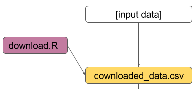
01_downloaded_data.csv: 01_download.R
    $(R_CMD) 01_download.R`

Syntax:

VAR = value

Example:

R_CMD = R CMD BATCH  --no-save --no-restore --slave --no-timing

# Macros

R_CMD = R CMD BATCH  --no-save --no-restore --slave --no-timing

# Targets

all: 01_downloaded_data.csv

01_downloaded_data.csv: 01_download.R makefile
    $(R_CMD) 01_download.R

# Macros

R_CMD = R CMD BATCH  --no-save --no-restore --slave --no-timing

# Targets

all: 03_model_output.Rds

01_downloaded_data.csv: 01_download.R makefile
    $(R_CMD) 01_download.R

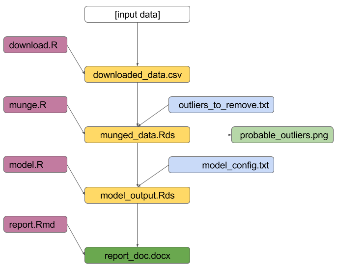
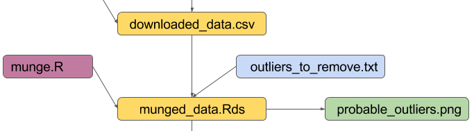
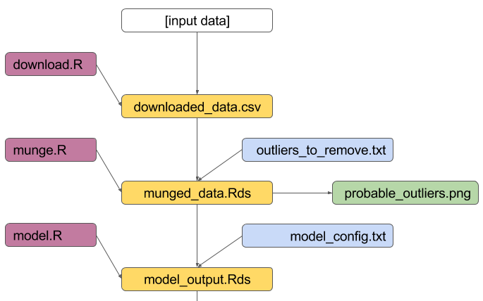
02_munged_data.Rds: 02_munge.R 01_downloaded_data.csv outliers_to_remove.txt
    $(R_CMD) 02_munge.R

03_model_output.Rds: 03_model.R 02_munged_data.Rds model_config.txt
    $(R_CMD) 03_model.R

# Macros

R_CMD = R CMD BATCH  --no-save --no-restore --slave --no-timing
R_SCRIPT = R --no-save --no-restore --no-init-file --no-site-file
SET_R_LIBS = .libPaths(c('~/Documents/R/win-library/3.2', \
                         'C:/Program Files/R/R-3.2.2/library'));
# Targets

all: 04_report_doc.docx

01_downloaded_data.csv: 01_download.R makefile
    $(R_CMD) 01_download.R

02_munged_data.Rds: 02_munge.R 01_downloaded_data.csv outliers_to_remove.txt
    $(R_CMD) 02_munge.R

03_model_output.Rds: 03_model.R 02_munged_data.Rds model_config.txt
    $(R_CMD) 03_model.R

04_report_doc.docx: 04_report.Rmd 03_model_output.Rds
    ${R_SCRIPT} -e "${SET_R_LIBS} \
                  knitr::knit(inp='04_report.Rmd', out='04_report.md')"
    pandoc 04_report.md --to docx --output 04_report_doc.docx

clean:
    rm -f *.Rout
    rm -f 04_report.md

Readable

• readable code
• traceable data flow

Self-contained

• complete from data to reports
• dependencies are embedded

Incorruptible

• judicious redundancy
• code versioning
• automated data flow