Goals for today's workshop

• GLM: basic understanding of lake model
• GLMr: run GLM from R, keep up-to-date version of GLM
• glmtools: reproducible model results handling and visualizations

The GLM model has been developed as an initiative of the Global Lake Ecological Observatory Network (GLEON) and in collaboration with the Aquatic Ecosystem Modelling Network (AEMON) that started in 2010. The model was first introduced in Leipzig at the 2nd Lake Ecosystem Modelling Symposium in 2012, and has since developed rapidly with application to numerous lakes within the GLEON network and beyond.

Source code available at http://github.com/GLEON/GLM-source

GLMr holds the current version of the "General Lake Model",
and can run the model on all platforms (windows, mac, linux) directly from R

glmtools is available on the GRAN repository.

install.packages(c("GLMr", "glmtools"), repos = c("http://owi.usgs.gov/R", 
    getOption("repos")))

More information can be found here.

GLMr Code in R:

library(GLMr)

glm_version()

nml_template_path()

Explanation

• load the GLMr package in R

• get the current version of GLM

• find the included example glm.nml

GLMr Code in R:

• run the GLM model on your computer

run_glm(sim_folder)

       ------------------------------------------------
       |  General Lake Model (GLM)   Version 2.1.8    |
       ------------------------------------------------
nDays 0 timestep 3600.000000
Maximum lake depth is 9.753600
Wall clock start time :  Mon Mar 07 16:28:55 2016
Simulation begins...
Wall clock finish time : Mon Mar 07 16:28:55 2016
Wall clock runtime 0 seconds : 00:00:00 [hh:mm:ss]

------------------------------------------------
              Run Complete
Reading config from glm2.nml
No WQ config
No diffuser data, setting default values
simulation complete. 

citation("GLMr")

## 
## To cite GLM in publications use:
## 
##   Hipsey, M.R., Bruce, L.C., Hamilton, D.P., 2013.
##   GLM General Lake Model. Model Overview and User
##   Information. The University of Western Australia
##   Technical Manual, Perth, Australia.
## 
## A BibTeX entry for LaTeX users is
## 
##   @Article{,
##     author = {Matthew R. Hipsey and Louise C. Bruce and David P. Hamilton},
##     title = {GLM General Lake Model. Model Overview and User Information},
##     journal = {The University of Western Australia Technical Manual, Perth, Australia},
##     year = {2013},
##   }
## 
## As GLM changes, this package will change with it, and
## the citation may change too. Find GLM version with
## 'glm_version()'.

Explanation

• Get the current citation for GLM

glmtools includes basic functions for calculating physical derivatives and thermal properties of model output, and plotting functionality. glmtools uses GLMr to run GLM

Goals
- understand model inputs
- run model
- visualize results

• Excercise: create and find your example folder

I am going to use a temporary directory, but you can pick any empty directory you want

library(glmtools)

tmp_run_dir = file.path(tempdir(), "glm_egs")
tmp_run_dir

## [1] "/var/folders/y_/1qp06xmj2ws0t8kv54q8wxgh0000gp/T//Rtmp2Q7O7H/glm_egs"

dir.create(tmp_run_dir)

• Navigate to that directory in your file finder

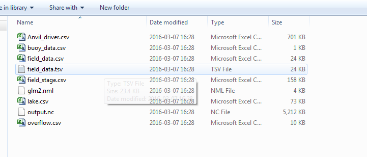
Now run the run_example_sim command and see the files created

run_example_sim(tmp_run_dir, verbose = FALSE)

## [1] "/var/folders/y_/1qp06xmj2ws0t8kv54q8wxgh0000gp/T//Rtmp2Q7O7H/glm_egs"

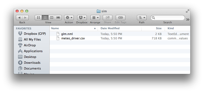
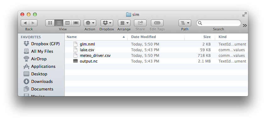
You should have a directory that looks like this

• load glmtools

• specify location of glm.nml file

• read glm.nml file into R

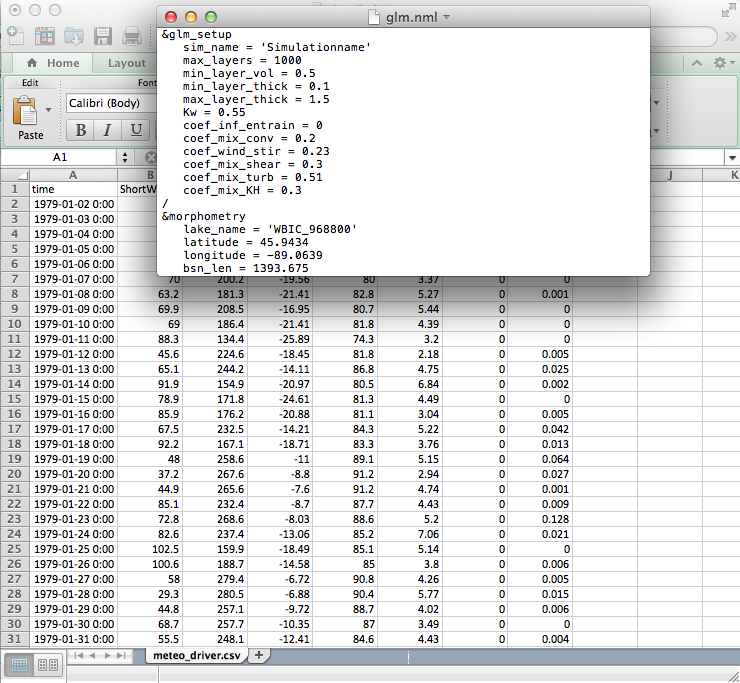
• print (view) the contents of the nml file

library(glmtools)
nml_file <- file.path(tmp_run_dir, "glm2.nml")
nml <- read_nml(nml_file)
nml

## &glm_setup
##    sim_name = 'GLMSimulation'
##    max_layers = 500
##    min_layer_vol = 0.025
##    min_layer_thick = 0.5
##    max_layer_thick = 1.5
##    Kw = 0.55
##    coef_mix_conv = 0.125
##    coef_wind_stir = 0.23
##    coef_mix_shear = 0.2
##    coef_mix_turb = 0.51
##    coef_mix_KH = 0.3
##    coef_mix_hyp = 0.5
## /
## &morphometry
##    lake_name = 'Anvil'
##    latitude = 32
##    longitude = 35
##    bsn_len = 21000
##    bsn_wid = 13000
##    bsn_vals = 15
##    H = 510.5363, 511.23299, 511.92967, 512.62636, 513.32304, 514.01973, 514.71641, 515.4131, 516.10979, 516.80647, 517.50316, 518.19984, 518.89653, 519.59321, 520.2899
##    A = 0, 108964, 217929, 326893, 435858, 544822.5, 653787, 762751, 871716, 980680, 1089645, 1198609, 1307574, 1416538, 1525503
## /
## &time
##    timefmt = 2
##    start = '2011-04-01 00:00:00'
##    stop = '2011-09-02 00:00:00'
##    dt = 3600
##    timezone = 7
## /
## &output
##    out_dir = '.'
##    out_fn = 'output'
##    nsave = 24
##    csv_lake_fname = 'lake'
##    csv_point_nlevs = 0
##    csv_point_fname = 'WQ_'
##    csv_point_at = 17
##    csv_point_nvars = 2
##    csv_point_vars = 'temp','salt','OXY_oxy'
##    csv_outlet_allinone = .false.
##    csv_outlet_fname = 'outlet_'
##    csv_outlet_nvars = 3
##    csv_outlet_vars = 'flow','temp','salt','OXY_oxy'
##    csv_ovrflw_fname = 'overflow'
## /
## &init_profiles
##    lake_depth = 9.7536
##    num_depths = 3
##    the_depths = 0, 1.2, 9.7536
##    the_temps = 12, 10, 7
##    the_sals = 0, 0, 0
##    num_wq_vars = 6
##    wq_names = 'OGM_don','OGM_pon','OGM_dop','OGM_pop','OGM_doc','OGM_poc'
##    wq_init_vals = 1.1, 1.2, 1.3, 1.2, 1.3, 2.1, 2.2, 2.3, 1.2, 1.3, 3.1, 3.2, 3.3, 1.2, 1.3, 4.1, 4.2, 4.3, 1.2, 1.3, 5.1, 5.2, 5.3, 1.2, 1.3, 6.1, 6.2, 6.3, 1.2, 1.3
## /
## &meteorology
##    met_sw = .true.
##    lw_type = 'LW_IN'
##    rain_sw = .false.
##    snow_sw = .false.
##    atm_stab = .false.
##    catchrain = .false.
##    rad_mode = 1
##    albedo_mode = 1
##    cloud_mode = 4
##    subdaily = .false.
##    meteo_fl = 'Anvil_driver.csv'
##    wind_factor = 1
##    sw_factor = 1
##    lw_factor = 1
##    at_factor = 1
##    rh_factor = 1
##    rain_factor = 1
##    ce = 0.0013
##    ch = 0.0013
##    cd = 0.00108
##    rain_threshold = 0.01
##    runoff_coef = 0.3
## /
## &bird_model
##    AP = 973
##    Oz = 0.279
##    WatVap = 1.1
##    AOD500 = 0.033
##    AOD380 = 0.038
##    Albedo = 0.2
## /
## &inflow
##    num_inflows = 0
##    names_of_strms = 'Riv1','Riv2'
##    subm_flag = .false.
##    strm_hf_angle = 65, 65
##    strmbd_slope = 2, 2
##    strmbd_drag = 0.016, 0.016
##    inflow_factor = 1, 1
##    inflow_fl = 'inflow_1.csv','inflow_2.csv'
##    inflow_varnum = 4
##    inflow_vars = 'FLOW','TEMP','SALT','OXY_oxy','SIL_rsi','NIT_amm','NIT_nit','PHS_frp','OGM_don','OGM_pon','OGM_dop','OGM_pop','OGM_doc','OGM_poc','PHY_green','PHY_crypto','PHY_diatom'
## /
## &outflow
##    num_outlet = 0
##    flt_off_sw = .false.
##    outl_elvs = -215.5
##    bsn_len_outl = 799
##    bsn_wid_outl = 399
##    outflow_fl = 'outflow.csv'
##    outflow_factor = 0.8
## /
## &snowice
##    snow_albedo_factor = 1
##    snow_rho_max = 300
##    snow_rho_min = 50
## /
## &sed_heat
##    sed_temp_mean = 9.7
##    sed_temp_amplitude = 2.7
##    sed_temp_peak_doy = 242.5
## /

• get values for specific parameters

get_nml_value(nml, "sim_name")

## [1] "GLMSimulation"

get_nml_value(nml, "Kw")

## [1] 0.55

• plot meteorological drivers for simulation

plot_meteo(nml_file)

• set simulation folder for GLM

• run GLM model

basename(tmp_run_dir)

## [1] "glm_egs"

run_glm(tmp_run_dir)

## [1] 0

• set output results file

• plot water temperatures

nc_file <- file.path(tmp_run_dir, "output.nc")

plot_temp(file = nc_file, fig_path = "../images/temperature.png")

Goals
- validate/evaluate model outputs
- modify model parameters
- run simulation with modified parameters

• change parameter value
  
• view nml with change

nml <- set_nml(nml, arg_name = "Kw", arg_val = 1.05)

print(nml)

## &glm_setup
##    sim_name = 'GLMSimulation'
##    max_layers = 500
##    min_layer_vol = 0.025
##    min_layer_thick = 0.5
##    max_layer_thick = 1.5
##    Kw = 1.05
##    coef_mix_conv = 0.125
##    coef_wind_stir = 0.23
##    coef_mix_shear = 0.2
##    coef_mix_turb = 0.51
##    coef_mix_KH = 0.3
##    coef_mix_hyp = 0.5
## /
## &morphometry
##    lake_name = 'Anvil'
##    latitude = 32
##    longitude = 35
##    bsn_len = 21000
##    bsn_wid = 13000
##    bsn_vals = 15
##    H = 510.5363, 511.23299, 511.92967, 512.62636, 513.32304, 514.01973, 514.71641, 515.4131, 516.10979, 516.80647, 517.50316, 518.19984, 518.89653, 519.59321, 520.2899
##    A = 0, 108964, 217929, 326893, 435858, 544822.5, 653787, 762751, 871716, 980680, 1089645, 1198609, 1307574, 1416538, 1525503
## /
## &time
##    timefmt = 2
##    start = '2011-04-01 00:00:00'
##    stop = '2011-09-02 00:00:00'
##    dt = 3600
##    timezone = 7
## /
## &output
##    out_dir = '.'
##    out_fn = 'output'
##    nsave = 24
##    csv_lake_fname = 'lake'
##    csv_point_nlevs = 0
##    csv_point_fname = 'WQ_'
##    csv_point_at = 17
##    csv_point_nvars = 2
##    csv_point_vars = 'temp','salt','OXY_oxy'
##    csv_outlet_allinone = .false.
##    csv_outlet_fname = 'outlet_'
##    csv_outlet_nvars = 3
##    csv_outlet_vars = 'flow','temp','salt','OXY_oxy'
##    csv_ovrflw_fname = 'overflow'
## /
## &init_profiles
##    lake_depth = 9.7536
##    num_depths = 3
##    the_depths = 0, 1.2, 9.7536
##    the_temps = 12, 10, 7
##    the_sals = 0, 0, 0
##    num_wq_vars = 6
##    wq_names = 'OGM_don','OGM_pon','OGM_dop','OGM_pop','OGM_doc','OGM_poc'
##    wq_init_vals = 1.1, 1.2, 1.3, 1.2, 1.3, 2.1, 2.2, 2.3, 1.2, 1.3, 3.1, 3.2, 3.3, 1.2, 1.3, 4.1, 4.2, 4.3, 1.2, 1.3, 5.1, 5.2, 5.3, 1.2, 1.3, 6.1, 6.2, 6.3, 1.2, 1.3
## /
## &meteorology
##    met_sw = .true.
##    lw_type = 'LW_IN'
##    rain_sw = .false.
##    snow_sw = .false.
##    atm_stab = .false.
##    catchrain = .false.
##    rad_mode = 1
##    albedo_mode = 1
##    cloud_mode = 4
##    subdaily = .false.
##    meteo_fl = 'Anvil_driver.csv'
##    wind_factor = 1
##    sw_factor = 1
##    lw_factor = 1
##    at_factor = 1
##    rh_factor = 1
##    rain_factor = 1
##    ce = 0.0013
##    ch = 0.0013
##    cd = 0.00108
##    rain_threshold = 0.01
##    runoff_coef = 0.3
## /
## &bird_model
##    AP = 973
##    Oz = 0.279
##    WatVap = 1.1
##    AOD500 = 0.033
##    AOD380 = 0.038
##    Albedo = 0.2
## /
## &inflow
##    num_inflows = 0
##    names_of_strms = 'Riv1','Riv2'
##    subm_flag = .false.
##    strm_hf_angle = 65, 65
##    strmbd_slope = 2, 2
##    strmbd_drag = 0.016, 0.016
##    inflow_factor = 1, 1
##    inflow_fl = 'inflow_1.csv','inflow_2.csv'
##    inflow_varnum = 4
##    inflow_vars = 'FLOW','TEMP','SALT','OXY_oxy','SIL_rsi','NIT_amm','NIT_nit','PHS_frp','OGM_don','OGM_pon','OGM_dop','OGM_pop','OGM_doc','OGM_poc','PHY_green','PHY_crypto','PHY_diatom'
## /
## &outflow
##    num_outlet = 0
##    flt_off_sw = .false.
##    outl_elvs = -215.5
##    bsn_len_outl = 799
##    bsn_wid_outl = 399
##    outflow_fl = 'outflow.csv'
##    outflow_factor = 0.8
## /
## &snowice
##    snow_albedo_factor = 1
##    snow_rho_max = 300
##    snow_rho_min = 50
## /
## &sed_heat
##    sed_temp_mean = 9.7
##    sed_temp_amplitude = 2.7
##    sed_temp_peak_doy = 242.5
## /

• write changed glm.nml to file

• run GLM model

write_nml(glm_nml = nml, file = nml_file)

run_glm(tmp_run_dir)

## [1] 0

• double check nc_file path

• quickly visualize new temps

nc_file <- file.path(tmp_run_dir, "output.nc")
plot_temp(file = nc_file, fig_path = "../images/temperature2.png")

• find simulation variables

sim_vars(file = nc_file)

##         name    unit         longname
## 1       evap     m/s      evaporation
## 2  extc_coef unknown        extc_coef
## 3       hice                     hice
## 4      hsnow                    hsnow
## 5      hwice                    hwice
## 6        I_0                      I_0
## 7         NS                       NS
## 8     precip     m/s    precipitation
## 9        rad unknown  solar radiation
## 10       rho unknown          density
## 11      salt    g/kg         salinity
## 12      temp celsius      temperature
## 13     Tot_V      m3      lake volume
## 14    u_mean     m/s    mean velocity
## 15     u_orb     m/s orbital velocity
## 16         V      m3     layer volume
## 17      wind     m/s             wind

• quickly visualize other variables

plot_var(file = nc_file, var_name = "u_mean", fig_path = "../images/velocity.png")

• quickly compare to field data

field_file <- file.path(tmp_run_dir, "field_data.tsv")
plot_var_compare(nc_file, field_file, "temp", resample = TRUE, 
    fig_path = "../images/temp_compare.png")